Activation function

Cost function

Quote

The purpose of the activation function is to introduce non-linearity into the network … without a non-linear activation function … the network would behave just like a single-layer perceptron ($y=Wx+b$). And: Without non-linear activation function there is no need of deep network because a combination of linear functions can be reduced to a single linear function.

What happens without an activation function (or using linear ones)

Consider a neural network built of layers where every single layer is purely linear. That is, each neuron just does: $y=Wx+b$ with no nonlinearity in between.

• Layer 1: $x\mapsto W_{1}x+b_1$
• Layer 2: $(W_{1}x+b_1)\mapsto W_2(W_{1}x+b_1)+b_2=(W_2{W}_1)x+(W_2{b}_1+b_2)$
• And so on… You can see by induction that a composition of linear transformations is itself a linear transformation. So no matter how many layers you stack, the whole network reduces to one big linear map from input to output. That means:
• You lose all depth advantage.
• You cannot model any non-linear relationships.
• You might as well have a single-layer linear model (e.g. logistic regression or linear regression, depending on loss) to achieve exactly the same result.

Thus, to gain expressive power — to approximate complex, nonlinear functions — we must break this linearity somewhere. That’s exactly what activation functions (nonlinear ones) do.

Why do we need activation function in neural network?

Beyond just nonlinearity, activation functions serve several practical and theoretical roles:

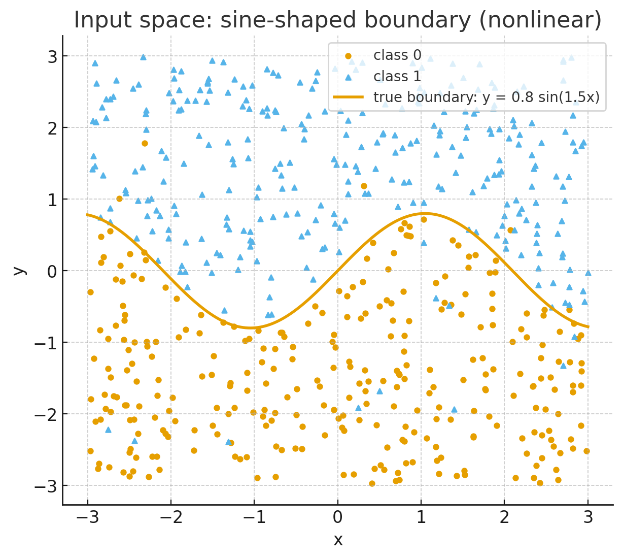
1. Allow modeling of nonlinear patterns Real-world data (images, audio, language, sensor data) often has patterns that are nonlinear: boundaries, curves, interactions. Activation functions let the network fit such patterns. 
2. Enable gradient-based learning (backpropagation) A good activation function is differentiable. That lets us compute gradients (via chain rule) and update weights. If an activation is non differentiable everywhere, training by gradient descent becomes problematic. 
3. Control signal scale and stability Activation functions (especially bounded ones like sigmoid or tanh) can help restrain large values, keep signals in a controlled range, and avoid numerical blowups. They impose nonlinear “squashing” or rectification which helps stabilize training.
4. Introduce saturations, thresholds, sparsity, etc. Depending on the design, activations can impose thresholds (e.g. zeroing out negatives), encourage sparse activations, or selectively “turn off” neurons. That helps in modularity and representational efficiency.
5. Universal approximation A theoretical guarantee: networks with at least one hidden layer using non‐polynomial activation functions (like sigmoid, ReLU) can approximate any continuous function on a compact domain (given enough neurons). This is the universal approximation theorem.

How activation function learns non linearity? Or What it means to learn nonlinearity?

Imagine trying to approximate a curve (say, a sine wave) using only straight line segments. If you only use straight lines with no ability to bend, your approximation is very limited. But if you allow “bend points” — nonlinear segments — you can piecewise fit the curve more closely.

In a neural network:

• The weights + biases define linear transforms.
• The activation functions let you “bend,” “threshold,” or “wrap” the signal, injecting nonlinearity. Thus, each neuron becomes a little nonlinear unit, and stacking many lets you carve out very flexible shapes in input space.

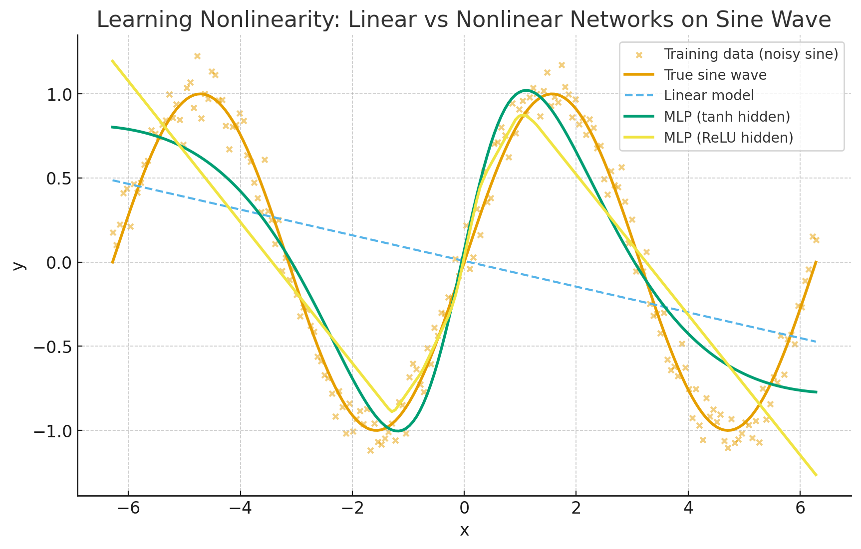MLP with tanh/ReLU hidden layer: bends and warps input space → learns the oscillations and tracks the sine wave much more closely.

How does the network learn this nonlinearity?

• Each hidden neuron applies: $a=\sigma (Wx+b)$
  • Linear part $Wx+b$= projection
  • Nonlinear part $\sigma =bend/warp$
• With training (via gradient descent), the network adjusts weights $W,b$ so that after nonlinear activations, the transformed space separates classes.
• Stacking layers = multiple nonlinear transformations → increasingly complex “warping” of input space.

---

Different activation functions.

Choosing a good activation function matters for learning dynamics, expressivity, and convergence.

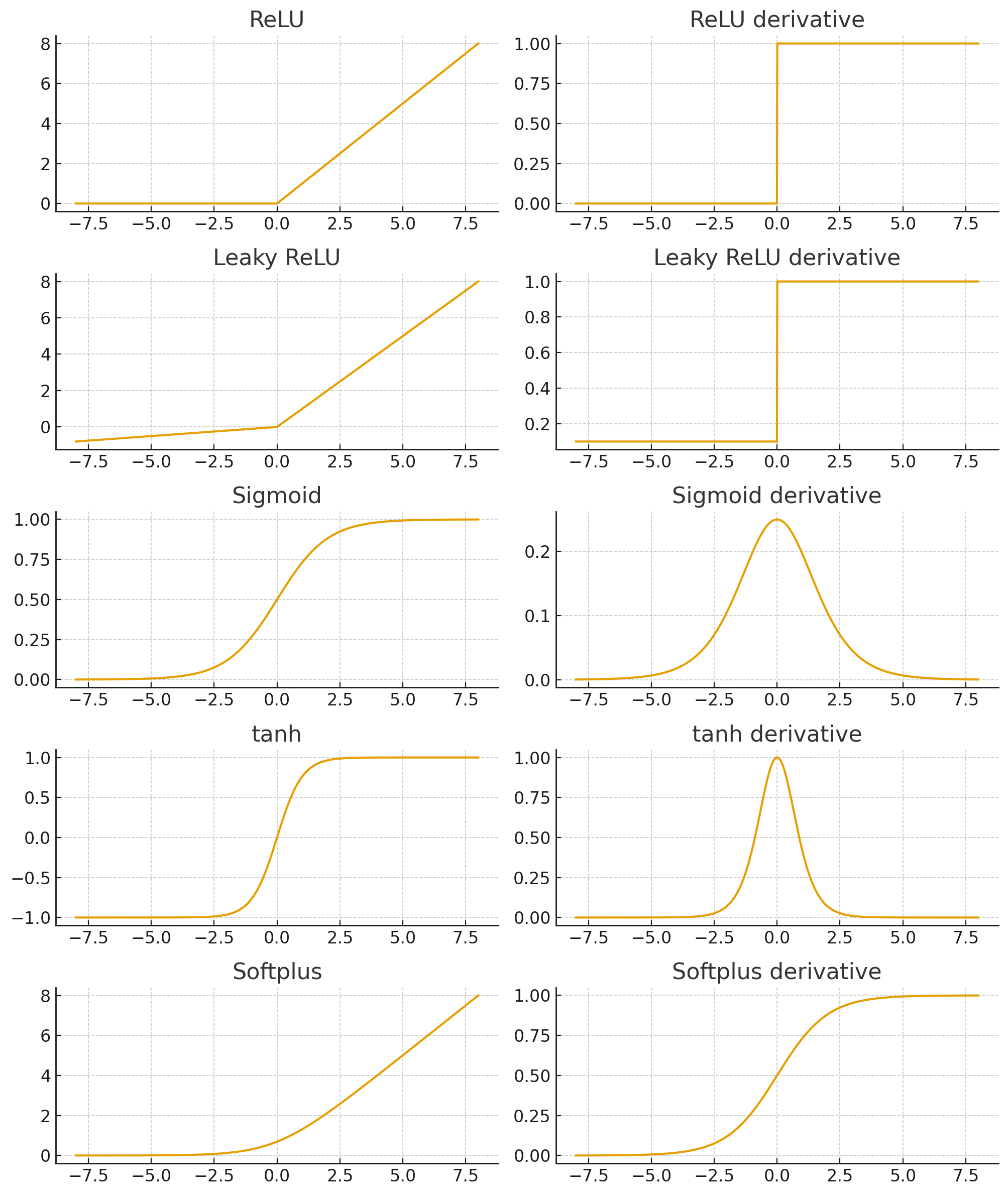
ReLU (Rectified Linear Unit)

$\mathrm{ReLU}(x)=\max (0,x)$ So:

• If $x>0$, output = x.
• If $x\le 0$, output = 0.
• Derivative: $\mathrm{ReLU}’(x)$ = 1 for x > 0, and 0 for x < 0.

Key properties

1. Sparse activation / “natural sparsity” Because negative inputs map to zero, many neurons will output zero, effectively “inactive,” which leads to a sparser representation and can help with efficiency or preventing overfitting. 
2. Computational simplicity It’s extremely cheap: just a threshold, no exponentials, no divisions, etc. 
3. Better gradient flow in deep networks Because the positive side is linear, gradient doesn’t vanish as layers increase. Empirically, using ReLU often accelerates convergence in deep nets compared to sigmoid/tanh. 
4. Biological plausibility (loose analogy) Some argue that neurons in biological brains don’t produce negative firing rates, so a rectified function is more plausible, though this is only a rough analogy.

Limitations & pitfalls (“Dying ReLU”, etc.)

• Dead / “dying ReLU”: If a neuron’s input becomes negative consistently and the weights update push it further negative, it can become stuck outputting zero forever (gradient = 0). Then it never recovers. 
• No negative output: This means the activation is not zero-centered, which sometimes slows convergence or introduces bias shift. (Because all activations are nonnegative, subsequent layers may have biased inputs.) 
• Unbounded output: Because for large x, output = x, there is no explicit bound, which may allow extremely large activations that need normalization (batch norm, etc.).

Because of these, many ReLU variants exist (Leaky ReLU, PReLU, etc.) that attempt to mitigate dying ReLUs.

---

Sigmoid function

$\sigma (z)=\frac{1}{1+e^{-z}}$

• Output of sigmoid is always in (0,1).
• Often interpreted as the probability of the “positive” class.
• Works great if you only have two classes $(sinceP(class1)=\sigma (z),andP(class0)=1-\sigma (z)$. 👉 But if you have K > 2 classes, just applying sigmoid to each logit doesn’t enforce they sum to 1. Each neuron independently decides “am I on or off?” — no competition.

Why sigmoid at the output doesn’t form a probability distribution

If you put a sigmoid on each of, say, 3 output neurons: $[\sigma (z1),\sigma (z2),\sigma (z3)]$

• Each entry is in (0,1).
• But the sum could be anything — e.g. 0.3 + 0.8 + 0.6 = 1.7 (invalid as probabilities).
• You can’t directly interpret them as “probability that input belongs to class 1, 2, or 3.” 👉 With sigmoid outputs, activations don’t naturally form a probability distribution**.

---

Softmax function

The softmax function takes a vector of raw scores (called logits, e.g. outputs of the last linear layer of a neural network) and converts them into a probability distribution.

$$\text{softmax}(z_i)=\frac{e^{z_i}}{{\sum }_{j=1}^K{e}^{z_j}},i=1,2,\dots ,K$$

Why do we need it?

• Neural networks end with numbers that can be positive or negative (logits).
• For classification, we need outputs that look like probabilities:
  • Non-negative
  • Sum to 1
• Linear outputs don’t satisfy this. Sigmoid works for binary class, but for multi-class, we need a generalization → softmax.
• Softmax probabilities are often paired with cross-entropy cost.
• This pairing has a special property: it simplifies gradients (avoids extra sigmoid-like shrinkage), making learning faster and numerically stable

Why not just normalize logits by dividing each by the sum of absolute values?

That wouldn’t preserve the exponential “competition” property; large logits should dominate more sharply than small ones.

Where is softmax applied in the network?

• Only at the output layer (in standard feedforward classifiers).
• Earlier layers use other activation functions (ReLU, sigmoid, tanh, etc.), because we don’t want every hidden neuron’s outputs to behave like a probability distribution.
• At the final layer, we want to map raw scores → probabilities, because classification = probability assignment.

---

Why not apply it everywhere throughout network?

If you applied softmax at every layer:

• Every hidden layer would force its outputs to sum to 1 → losing expressive power.
• Neurons couldn’t freely learn features, because they’d always be competing to form a probability distribution instead of just passing useful signals.
• Training would be unstable and inefficient. 👉 That’s why softmax is reserved for the final classification layer.

How softmax converts raw score into probability distribution?

Suppose the network outputs arbitrary real numbers: $z=[2.1,-1.5,0.3]$ These numbers can be negative or positive and have no constraint (they don’t add to 1). Clearly, they can’t be treated directly as probabilities.

Exponentiation

Larger logits get disproportionately larger after exponentiation → it sharpens differences between classes. Softmax first applies the exponential: $ez=[e2.1,e-1.5,e0.3]\approx [8.17,0.22,1.35]$

• This makes everything positive (good: probabilities can’t be negative).
• It also amplifies differences — larger logits grow disproportionately bigger.

Normalization (divide by the sum)

Now divide each term by the total sum:

$$\text{softmax}(z_i)=\frac{e^{z_i}}{{\sum }_{j=1}^K{e}^{z_j}},i=1,2,\dots ,K$$

Here, denominator = 8.17+0.22+1.35=9.74 So probabilities are: $[0.84,0.02,0.14]$

Intuition: Human brain parallel

Imagine you’re picking which dessert to eat: cake (score 3), fruit (score 1), or cookie (score 2).

• If you just picked max → always cake.
• But your brain sometimes explores alternatives.
• Softmax gives probabilistic preference:
  • Cake 70%, Cookie 20%, Fruit 10%.
    This balance between exploitation (pick best) and exploration (sometimes others) mirrors decision-making in brains.

✅ Summary intuition:

• Raw logits are “scores” saying how strong each class looks.
• Earlier layers are “feature extractors” → they shouldn’t be forced into probability distributions.
• Final layer = “decision-maker”
• Softmax = “competition game” among output neurons.
• Exponentiation sharpens competition.
• Normalization turns those sharpened scores into probabilities.

---

Comparing Sigmoid Vs Softmax

When to use which

• Sigmoid: binary classification (yes/no, spam/not spam).
• Softmax: multi-class classification (digit recognition 0–9, image category).
• Sigmoid with multiple outputs (independent): multi-label problems (e.g., “this photo contains dog=1, cat=1, car=0”). Here probabilities don’t need to sum to 1, because labels aren’t mutually exclusive.

We’ll compare sigmoid + cross-entropy (binary case) vs softmax + cross-entropy (multi-class case).

Sigmoid with cross-entropy (binary classification)

• Prediction: $\hat{y}=\sigma (z)=\frac{1}{1+e^{-z}}$
• Cross-entropy loss: $C=-(y\log \hat{y}+(1-y)\log (1-\hat{y}))$
• Gradient wrt logit $z$: $\frac{\partial C}{\partial z}=\hat{y}-y$ ✨ Notice: no extra σ′(z)σ′(z) term, because the derivative of sigmoid cancels with cross-entropy. This avoids vanishing gradients at the output layer.

Softmax with cross-entropy (multi-class classification)

• Prediction for class $i$: ${\hat{y}}_i=\frac{e^{z_i}}{{\sum }_{j=1}^K{e}^{z_j}},i=1,2,\dots ,K$
• Cross-entropy loss: $C=-{\sum }_{i=1}^K{y}_i\log {\hat{y}}_i$
• Gradient wrt logit $z$: $\frac{\partial C}{\partial z_i}={\hat{y}}_i-y_i$ ✨ Exactly the same simple form as sigmoid case! No messy chain rule terms survive — the math collapses nicely.

Why this is powerful

• Without cross-entropy, gradients involve sigmoid’(z) or softmax Jacobian, which shrink and cause vanishing gradients.
• With cross-entropy, the gradient becomes a simple difference between predicted and true probability.
• This gives stable, strong learning signals, especially at the output layer

Why sigmoid is local and softmax is not?

Sigmoid (locality property)

For the sigmoid: $a_j^L=\sigma \left(z_j^L\right)=\frac{1}{1+e^{-z_j^L}}$

• Each output $a_j^L$ depends only on its own input $z_j^L$ .
• Change $z_k^L$(for some $k\ne j$) → it does not affect $a_j^L$.
• This is why we say sigmoid is local: every neuron is independent.

Softmax (non-locality property)

For the softmax:

$$a_j^L=\frac{e^{z_j^L}}{{\sum }_{k=1}^K{e}^{z_k^L}},j=1,2,\dots ,K$$

• The numerator uses $z_j^L$​.
• But the denominator includes all logits $z_1^L,z_2^L,\dots ,z_K^L$.
• So, if you change any $z_k^L$ the denominator changes, and thus $a_j^L$​ changes too. 👉 That’s why softmax is non-local: the output probability for one class depends on all the others.

Why sigmoid and softmax curves are same?

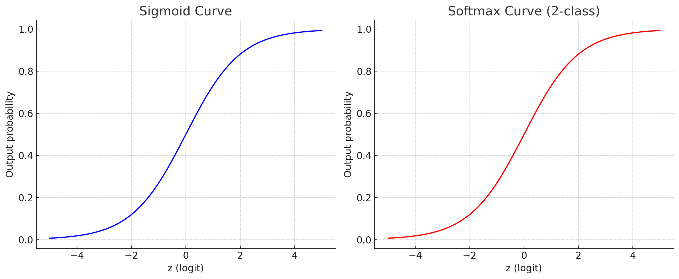
They look identical because softmax reduces to sigmoid in the binary case.

$$\text{Softmax}(z_i)=\frac{e^{z_i}}{{\sum }_{j=1}^K{e}^{z_j}}$$

With 2 classes, softmax essentially computes: $\text{Case: }K=2,z=[z_1,z_2]$

$${\hat{y}}_1=\frac{e^{z_1}}{e^{z_1}+e^{z_2}},{\hat{y}}_2=\frac{e^{z_2}}{e^{z_1}+e^{z_2}}$$

$\text{WLOG, let }{z}_2=0\text{ (we can shift logits without changing probabilities)}.$

$${\hat{y}}_1=\frac{e^{z_1}}{e^{z_1}+e^0}=\frac{e^{z_1}}{e^{z_1}+1}=\frac{1}{1+e^{-z_1}}=\sigma (z_1)$$ $$\therefore \text{Softmax}(z_1,0)=\sigma (z_1)$$

👉 That’s why the curves overlap: sigmoid is just the special case of softmax with two classes.