Learning is slow for sigmoid

investigation

Vanishing gradient problem

When people say “learning is slow for sigmoid”, they’re not talking about the external Learning Rate hyperparameter (η), but about the effective speed at which weights update inside the network.

We can see from this graph that when the neuron’s output is close to 1, the sigmoid curve gets very flat, and so σ′(z) gets very small.

• The blue curve is the sigmoid function.
• The orange dashed curve is its derivative.

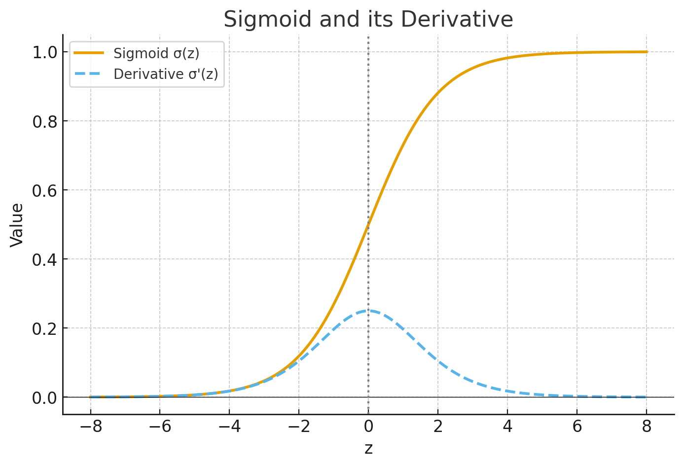
Notice how the derivative is largest at the center (near 0), but shrinks toward 0 at the extremes. 👉 That flattening is why gradients vanish, and learning becomes slow when sigmoid outputs are near 0 or 1.

Vanishing gradient problem in deep networks, showing how multiple layers make this slowdown compound.

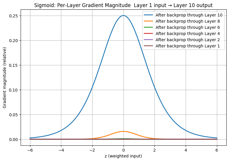
In the “compounded sigmoid derivatives” plot:

• Layer 10 (output) only carries 1 factor of σ′(z).
• Layer 1 (input) carries ~10 multiplications of σ′(z).
• Since σ′(z) ≤ 0.25, multiplying repeatedly makes the effective gradient near 0 for earlier layers
• The bell curve (gradient vs z) is tallest at the output layer.
• It shrinks layer by layer as you go back toward the input.

This means in deep sigmoid networks, early layers barely get learning signals. Later layers may update fine, but the front of the network “freezes.”

Why sigmoid is problematic

• Slow learning → derivatives vanish near 0/1 (as we saw).
• Vanishing gradients → in deep networks, signals die out quickly.
• Outputs not zero-centered → always positive, which biases gradient descent updates.
• Saturation → once neurons are stuck near 0/1, they hardly recover.

So, for deep hidden layers, sigmoid is usually a bad idea.

How can we address the learning slowdown?

Cross entropy cost function solves the slow down problem partially.

• Sigmoid vanishing gradients through depth (structural problem).
• Cross-entropy cost fixing slow learning at the output layer (local fix).

When using quadratic cost with sigmoid neurons: $C=\frac{1}{2}(y-a{)}^2,$ the gradient w.r.t weight is: $\frac{\partial C}{\partial w}=(a-y)\sigma ’(z)x.$

• Notice the σ′(z) term.
• If the sigmoid output a ≈ 0 or 1, then σ′(z) ≈ 0.
• Result: gradient ≈ 0 → learning is very slow even if the prediction is badly wrong

It turns out that we can solve the problem by replacing the quadratic cost with a different cost function, known as the cross-entropy. For more information reference this blog on Cost function. Cross-entropy cost function $C=-[y\ln a+(1-y)\ln (1-a)].$ Take the derivative: $\frac{\partial C}{\partial w}=(a-y)x.$

👉 The σ′(z) has disappeared!  That means:

• If the prediction is very wrong (say y=1, a≈0), the gradient is large → network corrects quickly.
• If the prediction is close to right (a≈y), the gradient is small → fine-tuning happens.

So cross-entropy matches gradient size to error size directly, instead of being throttled by sigmoid’s flat slope.

Side-by-side plot showing how gradients behave under quadratic vs cross-entropy cost when using sigmoid

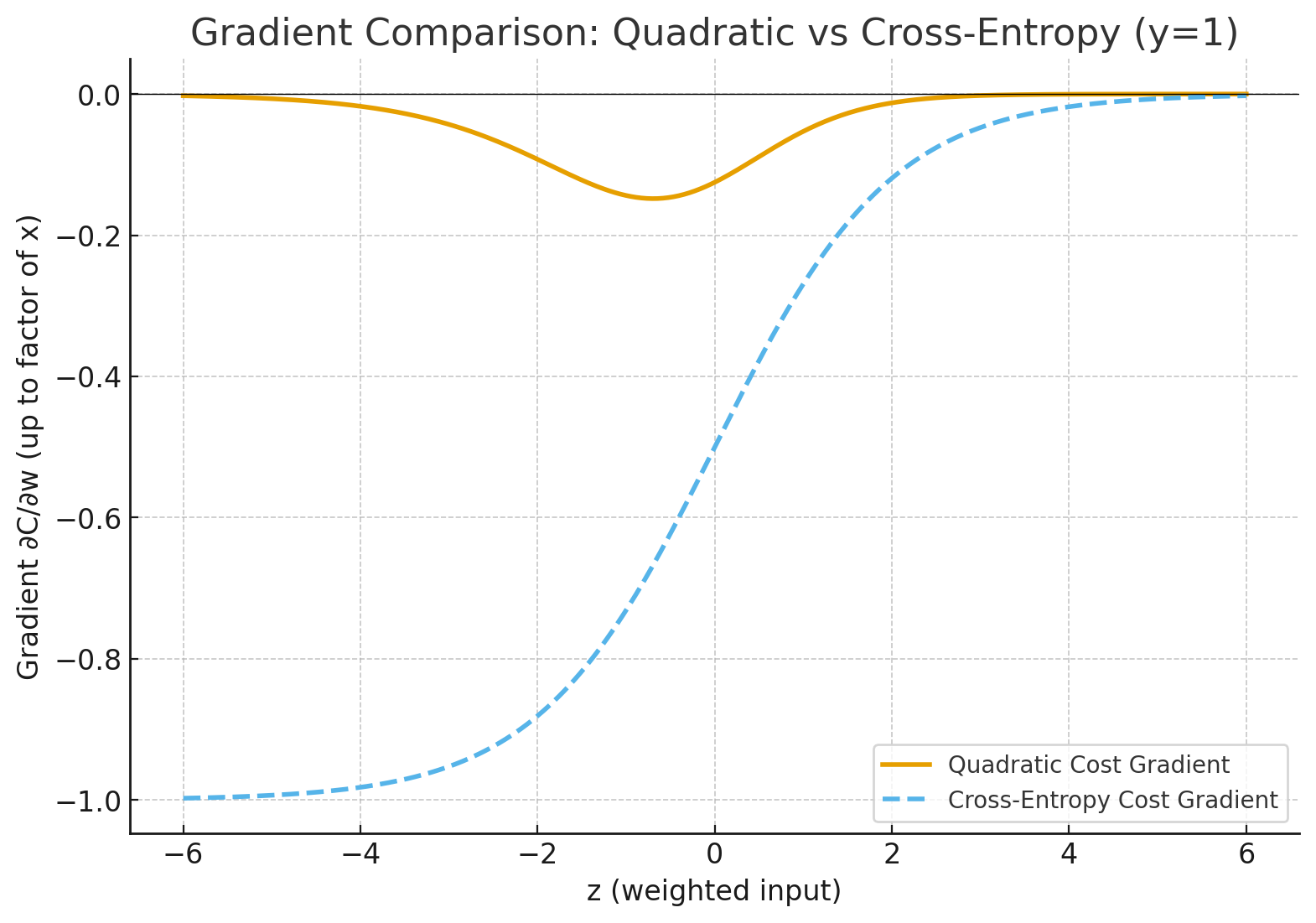
• Orange (Quadratic Cost): Gradient is tiny when the neuron is very wrong (large negative z, output near 0). That’s slow learning.
• Blue dashed (Cross-Entropy): Gradient stays strong when wrong, so the network corrects quickly.

Why vanishing gradients persist despite using cross entropy cost function?

• Cross-entropy only strengthens the starting signal at the output.
• As the gradient travels backward, hidden layers still multiply by $\sigma \prime (zl)$, which vanishes near 0 or 1.
• That’s why deep networks still need fixes like ReLU, batch norm, or residual connections.

Why keep sigmoid at all?

• Probabilistic interpretation → outputs in range (0,1). Perfect for representing probabilities.
  • Example: binary classification (spam vs not spam).
• Shallow networks or logistic regression → fine if the model is small, gradients don’t have time to vanish.

Modern practice

• Hidden layers: ReLU, Leaky ReLU, GELU, etc. (avoid vanishing gradient).
• Output layer:
  • Binary classification → Sigmoid.
  • Multi-class classification → Softmax.
  • Regression → often no activation (linear output).

---

👉 Summary:

• Don’t use sigmoid in hidden layers of deep nets.
• Use sigmoid at the output layer when you need probabilities for binary decisions.

---

Here’s the mathematical reasoning step by step:

1. Learning speed = size of gradients. In gradient descent, weights change according to $\Delta w=-\eta \frac{\partial C}{\partial w}.$ If the derivative (gradient) is very small, then even with a reasonable η, the weight barely moves. That’s “slow learning” .

2. Sigmoid derivative shrinks near 0 or 1. The sigmoid is $\sigma (z)=\frac{1}{1+e^{-z}},$ with derivative $\sigma ’(z)=\sigma (z)(1-\sigma (z)).$

   This derivative is maximum at 0.25 (when output = 0.5). As the neuron’s output saturates near 0 or 1, the slope flattens and $\sigma ’(z)\to 0$ .

3. Effect on gradients.
   The gradient of cost w.r.t. weights includes a factor of $\sigma ’(z)$. When $\sigma ’(z)$ is tiny, $\frac{\partial C}{\partial w}\approx 0,$ so the update step is negligible. That’s why the network learns slowly in those regions .

4. Why it matters.

   • For output neurons: if prediction is very close to 0 or 1 (but wrong), gradients vanish → slow correction.
   • For hidden neurons: saturation propagates vanishing gradients backward, making earlier layers barely learn .

👉 So “learning is slow for sigmoid” means: when sigmoid neurons saturate (outputs near 0 or 1), their gradients vanish, leading to tiny weight updates and hence very slow learning.